Reduced BSM1-Inspired Wastewater Treatment Model
![]()
![]()
This notebook implements a reduced BSM1-inspired activated sludge plant in Plugboard. BSM1, the Benchmark Simulation Model No. 1, is a standard wastewater-process benchmark built around ASM1 biological kinetics, pre-denitrification, and closed-loop control.
The full benchmark is too large and stiff for a clear teaching notebook, so this example focuses on the parts that best demonstrate Plugboard:
one anoxic reactor and one aerobic reactor
an internal recycle loop for nitrate return
a fixed return sludge stream from an ideal settler
PI control of nitrate and dissolved oxygen
dynamic influent disturbances, file-backed simulation output, and visualization
This is a control-topology tutorial, not a benchmark-faithful BSM1 reproduction. The notebook keeps the broad pre-denitrification story and the controller roles, but it also uses a reduced ASM1-inspired state vector and surrogate kinetics inside the reactors. The reported values are therefore illustrative tutorial outputs rather than benchmark-comparable KPIs, controller-tuning guidance, or publication-grade plant predictions.
The component classes and process assembly are shown directly in the notebook so readers can inspect the Plugboard model structure cell by cell.
Install and import dependencies
# Install plugboard and plotting dependencies for Google Colab
%pip install -q plugboard plotly pandas
from pathlib import Path
import math
import typing as _t

import pandas as pd
import plotly.graph_objects as go
from plotly.subplots import make_subplots
from pydantic import BaseModel, ConfigDict

from plugboard.component import Component
from plugboard.component import IOController as IO
from plugboard.connector import AsyncioConnector
from plugboard.diagram import MermaidDiagram, markdown_diagram
from plugboard.library import FileWriter
from plugboard.process import LocalProcess
from plugboard.schemas import ComponentArgsDict, ConnectorSpec
Which BSM1 ideas are preserved, reduced, or not included?
The table below makes the scope of the model explicit so the reader does not confuse this demo with a benchmark-grade BSM1 implementation. It preserves the plant architecture and control roles at a high level, but not the full benchmark dynamics or KPI machinery.
| Status | Aspect | Explanation |
|---|---|---|
| Preserved | Two PI loops | DO is manipulated through KLa and nitrate is manipulated through internal recycle flow, so the controller roles still match the standard BSM1 control story. |
| Preserved | Fixed return sludge flow | The return sludge stream is held constant, which matches the usual baseline BSM1 operating story. |
| Reduced | Bioreactor layout | The original five biological compartments are lumped into one anoxic and one aerobic reactor. |
| Reduced | Biology and state space | The notebook keeps a reduced ASM1-inspired state vector and surrogate kinetics, so the reactor biology is illustrative rather than benchmark-identical. |
| Reduced | Clarifier | The ten-layer settler is replaced by an ideal solids separator so the example stays readable and fast. |
| Reduced | Influent scenario | The influent uses a synthetic disturbed dry-weather profile instead of the standard benchmark influent files. |
| Not included | Standard BSM1 KPIs | This notebook does not compute the official EQI or OCI indices, so the results are not directly benchmark-comparable. |
Define the reduced BSM1 state and parameter set
We start with a small immutable stream object and a parameter bundle. The stream tracks the reduced ASM1-style state variables that will move through the Plugboard process.
STATE_FIELDS: tuple[str, ...] = (
    "s_s",
    "x_s",
    "x_bh",
    "x_ba",
    "s_o",
    "s_no",
    "s_nh",
    "s_nd",
    "x_nd",
)
PARTICULATE_FIELDS: tuple[str, ...] = ("x_s", "x_bh", "x_ba", "x_nd")
EPS = 1e-6


class WastewaterStream(BaseModel):
    """Represents a simplified ASM1 stream used in the reduced BSM1 demo."""

    model_config = ConfigDict(frozen=True)

    flow_m3_d: float
    s_s: float
    x_s: float
    x_bh: float
    x_ba: float
    s_o: float
    s_no: float
    s_nh: float
    s_nd: float
    x_nd: float

    @property
    def effluent_cod(self) -> float:
        return self.s_s + self.x_s

    @property
    def total_nitrogen(self) -> float:
        return self.s_nh + self.s_no + self.s_nd + self.x_nd


class BSM1Parameters(BaseModel):
    """Parameter set for the reduced BSM1 demo."""

    model_config = ConfigDict(frozen=True)

    dt_days: float = 5.0 / 1440.0
    total_days: float = 14.0
    v_anoxic_m3: float = 2000.0
    v_aerobic_m3: float = 4000.0
    q_in_avg_m3_d: float = 18446.0
    q_return_m3_d: float = 18446.0
    q_internal_bias_m3_d: float = 3.0 * 18446.0
    q_internal_min_m3_d: float = 0.5 * 18446.0
    q_internal_max_m3_d: float = 5.0 * 18446.0
    oxygen_saturation_g_m3: float = 8.0
    capture_efficiency: float = 0.995
    do_setpoint_g_m3: float = 2.0
    nitrate_setpoint_g_m3: float = 1.0
    kla_bias_d_inv: float = 120.0
    kla_min_d_inv: float = 30.0
    kla_max_d_inv: float = 240.0
    kla_rate_limit_d_inv_per_step: float = 20.0
    do_kp: float = 27.5
    do_ki: float = 110.0
    nitrate_kp: float = 2500.0
    nitrate_ki: float = 12000.0
    y_h: float = 0.67
    y_a: float = 0.24
    i_xb: float = 0.08
    mu_h_d_inv: float = 4.0
    mu_a_d_inv: float = 0.5
    b_h_d_inv: float = 0.3
    b_a_d_inv: float = 0.05
    k_s_g_m3: float = 10.0
    k_oh_g_m3: float = 0.2
    k_oa_g_m3: float = 0.4
    k_no_g_m3: float = 0.5
    k_nh_g_m3: float = 1.0
    k_h_d_inv: float = 3.0
    k_x_g_m3: float = 100.0
    k_a_d_inv: float = 0.08
    k_nd_g_m3: float = 1.0
    eta_g: float = 0.8
    eta_h: float = 0.4
    decay_to_xs_fraction: float = 0.35
    nitrification_oxygen_factor: float = 1.5

    @property
    def total_steps(self) -> int:
        return int(self.total_days / self.dt_days)
A plain-language guide to the wastewater variables
If you do not work in wastewater treatment every day, the stream fields can look opaque. The reduced model keeps only the variables needed to tell the control story.
flow_m3_d: total stream flow in cubic metres per day.s_s: readily biodegradable soluble substrate. You can think of this as the easiest food for the heterotrophic biomass to consume.x_s: slowly biodegradable particulate substrate. This is still organic matter, but it must hydrolyse before the biomass can use it.x_bh: heterotrophic biomass, the organisms that mainly remove organic carbon and can denitrify when oxygen is scarce.x_ba: autotrophic biomass, the nitrifiers that oxidise ammonium when oxygen is available.s_o: dissolved oxygen, the main controlled variable in the aerobic reactor.s_no: oxidised nitrogen, represented here as nitrate and nitrite together. The internal recycle loop sends this back to the anoxic zone for denitrification.s_nh: ammonium nitrogen, the reduced nitrogen form that the aerobic biology tries to oxidise.s_ndandx_nd: soluble and particulate organic nitrogen pools. These provide a simple way to keep nitrogen tied to the organic matter balance.
The notebook is still a reduced teaching model, but these variables are enough to connect the biology to the two feedback controllers and the main effluent trends.
Helper functions for reactor balances and initial conditions
The next cells keep the notebook readable by separating the low-level numerical helpers from the Plugboard components themselves.
def _stream_kwargs(stream: WastewaterStream) -> dict[str, float]:
    return {field: float(getattr(stream, field)) for field in STATE_FIELDS}


def _make_stream(flow_m3_d: float, values: dict[str, float]) -> WastewaterStream:
    return WastewaterStream(flow_m3_d=flow_m3_d, **values)


def _non_negative_stream(stream: WastewaterStream) -> WastewaterStream:
    return WastewaterStream(
        flow_m3_d=max(stream.flow_m3_d, EPS),
        **{field: max(getattr(stream, field), 0.0) for field in STATE_FIELDS},
    )


def _with_flow(stream: WastewaterStream, flow_m3_d: float) -> WastewaterStream:
    return WastewaterStream(flow_m3_d=max(flow_m3_d, EPS), **_stream_kwargs(stream))


def _blend_streams(streams: _t.Sequence[WastewaterStream]) -> WastewaterStream:
    total_flow = sum(stream.flow_m3_d for stream in streams)
    if total_flow <= EPS:
        return WastewaterStream(
            flow_m3_d=EPS,
            s_s=0.0,
            x_s=0.0,
            x_bh=0.0,
            x_ba=0.0,
            s_o=0.0,
            s_no=0.0,
            s_nh=0.0,
            s_nd=0.0,
            x_nd=0.0,
        )
    blended = {
        field: sum(stream.flow_m3_d * getattr(stream, field) for stream in streams) / total_flow
        for field in STATE_FIELDS
    }
    return _make_stream(total_flow, blended)


def _advance_stream(
    current: WastewaterStream,
    inflows: _t.Sequence[WastewaterStream],
    volume_m3: float,
    params: BSM1Parameters,
    kla_d_inv: float,
) -> WastewaterStream:
    mixed = _blend_streams(inflows)
    total_flow = mixed.flow_m3_d

    ss = max(current.s_s, 0.0)
    xs = max(current.x_s, 0.0)
    xbh = max(current.x_bh, 0.0)
    xba = max(current.x_ba, 0.0)
    so = max(current.s_o, 0.0)
    sno = max(current.s_no, 0.0)
    snh = max(current.s_nh, 0.0)
    snd = max(current.s_nd, 0.0)
    xnd = max(current.x_nd, 0.0)

    substrate_term = ss / (params.k_s_g_m3 + ss + EPS)
    oxygen_term_h = so / (params.k_oh_g_m3 + so + EPS)
    oxygen_term_a = so / (params.k_oa_g_m3 + so + EPS)
    anoxic_term = params.k_oh_g_m3 / (params.k_oh_g_m3 + so + EPS)
    nitrate_term = sno / (params.k_no_g_m3 + sno + EPS)
    ammonium_term = snh / (params.k_nh_g_m3 + snh + EPS)
    hydrolysis_term = xs / (params.k_x_g_m3 + xs + EPS)
    hydrolysis_drive = oxygen_term_h + params.eta_h * anoxic_term * nitrate_term
    organic_n_term = snd / (params.k_nd_g_m3 + snd + EPS)

    rho_aer_h = params.mu_h_d_inv * substrate_term * oxygen_term_h * xbh
    rho_anox_h = (
        params.eta_g * params.mu_h_d_inv * substrate_term * anoxic_term * nitrate_term * xbh
    )
    rho_auto = params.mu_a_d_inv * ammonium_term * oxygen_term_a * xba
    rho_decay_h = params.b_h_d_inv * xbh
    rho_decay_a = params.b_a_d_inv * xba
    rho_ammonification = params.k_a_d_inv * organic_n_term * xbh
    rho_hydrolysis = params.k_h_d_inv * hydrolysis_term * hydrolysis_drive * xbh
    rho_hydrolysis_n = (xnd / max(xs, EPS)) * rho_hydrolysis if xs > EPS else 0.0

    reactions = {
        "s_s": rho_hydrolysis - (rho_aer_h + rho_anox_h) / params.y_h,
        "x_s": -rho_hydrolysis + params.decay_to_xs_fraction * (rho_decay_h + rho_decay_a),
        "x_bh": rho_aer_h + rho_anox_h - rho_decay_h,
        "x_ba": rho_auto - rho_decay_a,
        "s_o": -((1.0 - params.y_h) / params.y_h) * rho_aer_h
        - params.nitrification_oxygen_factor * rho_auto
        + max(kla_d_inv, 0.0) * (params.oxygen_saturation_g_m3 - so),
        "s_no": (1.0 / params.y_a) * rho_auto
        - ((1.0 - params.y_h) / (2.86 * params.y_h)) * rho_anox_h,
        "s_nh": -(params.i_xb * (rho_aer_h + rho_anox_h))
        - ((1.0 / params.y_a) + params.i_xb) * rho_auto
        + rho_ammonification
        + params.i_xb * (rho_decay_h + rho_decay_a),
        "s_nd": -rho_ammonification + rho_hydrolysis_n,
        "x_nd": params.i_xb * (rho_decay_h + rho_decay_a) - rho_hydrolysis_n,
    }

    dilution = total_flow / volume_m3
    updated: dict[str, float] = {}
    current_values = _stream_kwargs(current)
    mixed_values = _stream_kwargs(mixed)
    for field in STATE_FIELDS:
        derivative = dilution * (mixed_values[field] - current_values[field]) + reactions[field]
        updated[field] = current_values[field] + params.dt_days * derivative

    return _non_negative_stream(_make_stream(total_flow, updated))
def _base_influent(params: BSM1Parameters) -> WastewaterStream:
    return WastewaterStream(
        flow_m3_d=params.q_in_avg_m3_d,
        s_s=69.5,
        x_s=202.32,
        x_bh=28.17,
        x_ba=0.0,
        s_o=0.0,
        s_no=0.0,
        s_nh=31.56,
        s_nd=6.95,
        x_nd=10.59,
    )


def _initial_anoxic_state(params: BSM1Parameters) -> WastewaterStream:
    return WastewaterStream(
        flow_m3_d=params.q_in_avg_m3_d + params.q_return_m3_d + params.q_internal_bias_m3_d,
        s_s=28.0,
        x_s=175.0,
        x_bh=2250.0,
        x_ba=110.0,
        s_o=0.15,
        s_no=1.1,
        s_nh=16.0,
        s_nd=3.4,
        x_nd=11.0,
    )


def _initial_aerobic_state(params: BSM1Parameters) -> WastewaterStream:
    return WastewaterStream(
        flow_m3_d=params.q_in_avg_m3_d + params.q_return_m3_d,
        s_s=8.0,
        x_s=110.0,
        x_bh=2100.0,
        x_ba=185.0,
        s_o=params.do_setpoint_g_m3,
        s_no=6.5,
        s_nh=2.0,
        s_nd=1.1,
        x_nd=7.0,
    )


def _initial_internal_recycle(params: BSM1Parameters) -> WastewaterStream:
    return _with_flow(_initial_aerobic_state(params), params.q_internal_bias_m3_d)


def _initial_settler_streams(
    params: BSM1Parameters,
) -> tuple[WastewaterStream, WastewaterStream, WastewaterStream]:
    aerobic = _initial_aerobic_state(params)
    feed = _with_flow(aerobic, params.q_in_avg_m3_d + params.q_return_m3_d)
    eff_flow = max(feed.flow_m3_d - params.q_return_m3_d, EPS)
    solids_to_return = params.capture_efficiency

    effluent_values = _stream_kwargs(feed)
    return_values = _stream_kwargs(feed)
    for field in PARTICULATE_FIELDS:
        feed_mass = getattr(feed, field) * feed.flow_m3_d
        effluent_values[field] = ((1.0 - solids_to_return) * feed_mass) / eff_flow
        return_values[field] = (solids_to_return * feed_mass) / params.q_return_m3_d

    return (
        feed,
        _non_negative_stream(_make_stream(eff_flow, effluent_values)),
        _non_negative_stream(_make_stream(params.q_return_m3_d, return_values)),
    )
Define the Plugboard components
This is the key part of the example. Each major unit operation and control element becomes a normal Plugboard component, with explicit inputs and outputs that we will later wire together with connectors.
class InfluentScenario(Component):
    """Generates a dynamic dry-weather-plus-disturbance influent profile."""

    io = IO(
        outputs=[
            "influent",
            "time_day",
            "do_setpoint",
            "nitrate_setpoint",
            "tick",
            "influent_flow",
            "influent_s_s",
            "influent_s_nh",
        ]
    )

    def __init__(self, params: BSM1Parameters, **kwargs: _t.Unpack[ComponentArgsDict]) -> None:
        super().__init__(**kwargs)
        self._params = params
        self._step_index = 0
        self._base = _base_influent(params)

    def _profile(self, time_day: float) -> WastewaterStream:
        q_scale = 1.0 + 0.08 * math.sin(2.0 * math.pi * time_day)
        q_scale += 0.04 * math.sin(4.0 * math.pi * time_day - 1.0)
        cod_scale = 1.0 + 0.10 * math.sin(2.0 * math.pi * (time_day - 0.15))
        nh_scale = 1.0 + 0.07 * math.sin(2.0 * math.pi * (time_day - 0.10))

        if 4.0 <= time_day < 6.0:
            nh_scale += 0.25
        if 8.0 <= time_day < 10.0:
            q_scale += 0.35
            cod_scale -= 0.10
            nh_scale -= 0.05
        if 11.0 <= time_day < 12.5:
            cod_scale += 0.20
            nh_scale += 0.10

        return WastewaterStream(
            flow_m3_d=self._base.flow_m3_d * q_scale,
            s_s=self._base.s_s * cod_scale,
            x_s=self._base.x_s * cod_scale,
            x_bh=self._base.x_bh,
            x_ba=self._base.x_ba,
            s_o=0.0,
            s_no=0.0,
            s_nh=self._base.s_nh * nh_scale,
            s_nd=self._base.s_nd * nh_scale,
            x_nd=self._base.x_nd * nh_scale,
        )

    async def step(self) -> None:
        if self._step_index >= self._params.total_steps:
            await self.io.close()
            return

        time_day = self._step_index * self._params.dt_days
        self.influent = self._profile(time_day)
        self.time_day = time_day
        self.do_setpoint = self._params.do_setpoint_g_m3
        self.nitrate_setpoint = self._params.nitrate_setpoint_g_m3
        self.tick = self._step_index
        self.influent_flow = self.influent.flow_m3_d
        self.influent_s_s = self.influent.s_s
        self.influent_s_nh = self.influent.s_nh

        self._step_index += 1


class PIController(Component):
    """Simple PI controller with output limits and anti-windup."""

    io = IO(inputs=["measurement", "setpoint", "tick"], outputs=["control_signal"])

    def __init__(
        self,
        kp: float,
        ki: float,
        bias: float,
        lower: float,
        upper: float,
        dt_days: float,
        **kwargs: _t.Unpack[ComponentArgsDict],
    ) -> None:
        super().__init__(**kwargs)
        self._kp = kp
        self._ki = ki
        self._bias = bias
        self._lower = lower
        self._upper = upper
        self._dt_days = dt_days
        self._integral = 0.0

    async def step(self) -> None:
        error = self.setpoint - self.measurement
        proposed_integral = self._integral + self._ki * error * self._dt_days
        raw_output = self._bias + (self._kp * error) + proposed_integral
        bounded_output = min(max(raw_output, self._lower), self._upper)

        should_integrate = self._lower < raw_output < self._upper
        should_integrate = should_integrate or (raw_output <= self._lower and error > 0.0)
        should_integrate = should_integrate or (raw_output >= self._upper and error < 0.0)
        if should_integrate:
            self._integral = proposed_integral
            raw_output = self._bias + (self._kp * error) + self._integral
            bounded_output = min(max(raw_output, self._lower), self._upper)

        self.control_signal = bounded_output
class AnoxicReactor(Component):
    """Reduced anoxic bioreactor with ASM1-inspired nitrogen and COD dynamics."""

    io = IO(
        inputs=["influent", "internal_recycle", "return_sludge", "tick"],
        outputs=["mixed_liquor", "s_no", "anoxic_s_s"],
    )

    def __init__(
        self,
        params: BSM1Parameters,
        initial_state: WastewaterStream,
        **kwargs: _t.Unpack[ComponentArgsDict],
    ) -> None:
        super().__init__(**kwargs)
        self._params = params
        self._stream_state = initial_state

    async def step(self) -> None:
        self._stream_state = _advance_stream(
            current=self._stream_state,
            inflows=[self.influent, self.internal_recycle, self.return_sludge],
            volume_m3=self._params.v_anoxic_m3,
            params=self._params,
            kla_d_inv=0.0,
        )
        self.mixed_liquor = self._stream_state
        self.s_no = self._stream_state.s_no
        self.anoxic_s_s = self._stream_state.s_s


class AerobicReactor(Component):
    """Reduced aerobic reactor with explicit aeration and internal recycle split."""

    io = IO(
        inputs=["feed", "recycle_flow", "kla", "tick"],
        outputs=[
            "to_settler",
            "internal_recycle",
            "s_o",
            "aerobic_s_nh",
            "internal_recycle_flow",
            "applied_kla",
        ],
    )

    def __init__(
        self,
        params: BSM1Parameters,
        initial_state: WastewaterStream,
        **kwargs: _t.Unpack[ComponentArgsDict],
    ) -> None:
        super().__init__(**kwargs)
        self._params = params
        self._stream_state = initial_state
        self._kla_state = params.kla_bias_d_inv

    async def step(self) -> None:
        requested_kla = min(
            max(self.kla, self._params.kla_min_d_inv),
            self._params.kla_max_d_inv,
        )
        kla_delta = requested_kla - self._kla_state
        max_delta = self._params.kla_rate_limit_d_inv_per_step
        if kla_delta > max_delta:
            self._kla_state += max_delta
        elif kla_delta < -max_delta:
            self._kla_state -= max_delta
        else:
            self._kla_state = requested_kla

        self._stream_state = _advance_stream(
            current=self._stream_state,
            inflows=[self.feed],
            volume_m3=self._params.v_aerobic_m3,
            params=self._params,
            kla_d_inv=self._kla_state,
        )

        recycle_flow = min(
            max(self.recycle_flow, self._params.q_internal_min_m3_d),
            self._params.q_internal_max_m3_d,
        )
        settler_flow = max(self.feed.flow_m3_d - recycle_flow, EPS)

        self.internal_recycle = _with_flow(self._stream_state, recycle_flow)
        self.to_settler = _with_flow(self._stream_state, settler_flow)
        self.s_o = self._stream_state.s_o
        self.aerobic_s_nh = self._stream_state.s_nh
        self.internal_recycle_flow = recycle_flow
        self.applied_kla = self._kla_state


class IdealSettler(Component):
    """Ideal solids separator used as a pedagogical replacement for the 10-layer clarifier."""

    io = IO(
        inputs=["feed", "tick"],
        outputs=[
            "return_sludge",
            "effluent_cod",
            "effluent_s_s",
            "effluent_s_nh",
            "effluent_s_no",
            "effluent_total_n",
            "return_sludge_x_bh",
        ],
    )

    def __init__(self, params: BSM1Parameters, **kwargs: _t.Unpack[ComponentArgsDict]) -> None:
        super().__init__(**kwargs)
        self._params = params

    async def step(self) -> None:
        effluent_flow = max(self.feed.flow_m3_d - self._params.q_return_m3_d, EPS)
        effluent_values = _stream_kwargs(self.feed)
        return_values = _stream_kwargs(self.feed)

        for field in PARTICULATE_FIELDS:
            feed_mass = getattr(self.feed, field) * self.feed.flow_m3_d
            effluent_values[field] = (
                (1.0 - self._params.capture_efficiency) * feed_mass / effluent_flow
            )
            return_values[field] = (
                self._params.capture_efficiency * feed_mass / self._params.q_return_m3_d
            )

        effluent = _non_negative_stream(_make_stream(effluent_flow, effluent_values))
        self.return_sludge = _non_negative_stream(
            _make_stream(self._params.q_return_m3_d, return_values)
        )
        self.effluent_cod = effluent.effluent_cod
        self.effluent_s_s = effluent.s_s
        self.effluent_s_nh = effluent.s_nh
        self.effluent_s_no = effluent.s_no
        self.effluent_total_n = effluent.total_nitrogen
        self.return_sludge_x_bh = self.return_sludge.x_bh
Assemble the Plugboard process
Once the components are defined, the rest is standard Plugboard work: instantiate the components, create connectors, and build a LocalProcess. The writer is connected directly to scalar outputs from the process components, so a few extra outputs exist only to make file writing and plotting explicit inside the notebook.
def build_process(
    output_path: str | Path = "bsm1_results.csv",
    params: BSM1Parameters | None = None,
) -> LocalProcess:
    """Builds the reduced BSM1 demo process."""

    params = params or BSM1Parameters()
    initial_anoxic = _initial_anoxic_state(params)
    initial_aerobic = _initial_aerobic_state(params)
    initial_internal = _initial_internal_recycle(params)
    initial_settler_feed, _, initial_return = _initial_settler_streams(params)

    def connect(source: str, target: str) -> AsyncioConnector:
        return AsyncioConnector(spec=ConnectorSpec(source=source, target=target))

    influent = InfluentScenario(name="influent", params=params)
    nitrate_controller = PIController(
        name="nitrate_controller",
        kp=params.nitrate_kp,
        ki=params.nitrate_ki,
        bias=params.q_internal_bias_m3_d,
        lower=params.q_internal_min_m3_d,
        upper=params.q_internal_max_m3_d,
        dt_days=params.dt_days,
        initial_values={
            "measurement": [initial_anoxic.s_no],
            "setpoint": [params.nitrate_setpoint_g_m3],
        },
    )
    do_controller = PIController(
        name="do_controller",
        kp=params.do_kp,
        ki=params.do_ki,
        bias=params.kla_bias_d_inv,
        lower=params.kla_min_d_inv,
        upper=params.kla_max_d_inv,
        dt_days=params.dt_days,
        initial_values={
            "measurement": [initial_aerobic.s_o],
            "setpoint": [params.do_setpoint_g_m3],
        },
    )
    anoxic = AnoxicReactor(
        name="anoxic_reactor",
        params=params,
        initial_state=initial_anoxic,
        initial_values={
            "internal_recycle": [initial_internal],
            "return_sludge": [initial_return],
        },
    )
    aerobic = AerobicReactor(
        name="aerobic_reactor",
        params=params,
        initial_state=initial_aerobic,
        initial_values={
            "feed": [initial_anoxic],
            "recycle_flow": [params.q_internal_bias_m3_d],
            "kla": [params.kla_bias_d_inv],
        },
    )
    settler = IdealSettler(
        name="ideal_settler",
        params=params,
        initial_values={"feed": [initial_settler_feed]},
    )
    writer = FileWriter(
        name="writer",
        path=str(output_path),
        field_names=[
            "time_day_out",
            "influent_flow",
            "influent_s_s",
            "influent_s_nh",
            "anoxic_s_no",
            "anoxic_s_s",
            "aerobic_s_o",
            "aerobic_s_nh",
            "effluent_cod",
            "effluent_s_s",
            "effluent_s_nh",
            "effluent_s_no",
            "effluent_total_n",
            "return_sludge_x_bh",
            "internal_recycle_flow",
            "kla_out",
            "requested_kla_out",
            "do_setpoint_out",
            "nitrate_setpoint_out",
        ],
    )

    components = [
        influent,
        nitrate_controller,
        do_controller,
        anoxic,
        aerobic,
        settler,
        writer,
    ]
    connectors = [
        connect("influent.influent", "anoxic_reactor.influent"),
        connect("influent.tick", "nitrate_controller.tick"),
        connect("influent.tick", "do_controller.tick"),
        connect("influent.tick", "anoxic_reactor.tick"),
        connect("influent.tick", "aerobic_reactor.tick"),
        connect("influent.tick", "ideal_settler.tick"),
        connect("influent.time_day", "writer.time_day_out"),
        connect("influent.influent_flow", "writer.influent_flow"),
        connect("influent.influent_s_s", "writer.influent_s_s"),
        connect("influent.influent_s_nh", "writer.influent_s_nh"),
        connect("influent.do_setpoint", "do_controller.setpoint"),
        connect("influent.do_setpoint", "writer.do_setpoint_out"),
        connect("influent.nitrate_setpoint", "nitrate_controller.setpoint"),
        connect("influent.nitrate_setpoint", "writer.nitrate_setpoint_out"),
        connect("anoxic_reactor.mixed_liquor", "aerobic_reactor.feed"),
        connect("anoxic_reactor.s_no", "nitrate_controller.measurement"),
        connect("anoxic_reactor.s_no", "writer.anoxic_s_no"),
        connect("anoxic_reactor.anoxic_s_s", "writer.anoxic_s_s"),
        connect("nitrate_controller.control_signal", "aerobic_reactor.recycle_flow"),
        connect("aerobic_reactor.internal_recycle", "anoxic_reactor.internal_recycle"),
        connect("aerobic_reactor.to_settler", "ideal_settler.feed"),
        connect("aerobic_reactor.s_o", "do_controller.measurement"),
        connect("aerobic_reactor.s_o", "writer.aerobic_s_o"),
        connect("aerobic_reactor.aerobic_s_nh", "writer.aerobic_s_nh"),
        connect("aerobic_reactor.internal_recycle_flow", "writer.internal_recycle_flow"),
        connect("aerobic_reactor.applied_kla", "writer.kla_out"),
        connect("do_controller.control_signal", "aerobic_reactor.kla"),
        connect("do_controller.control_signal", "writer.requested_kla_out"),
        connect("ideal_settler.return_sludge", "anoxic_reactor.return_sludge"),
        connect("ideal_settler.effluent_cod", "writer.effluent_cod"),
        connect("ideal_settler.effluent_s_s", "writer.effluent_s_s"),
        connect("ideal_settler.effluent_s_nh", "writer.effluent_s_nh"),
        connect("ideal_settler.effluent_s_no", "writer.effluent_s_no"),
        connect("ideal_settler.effluent_total_n", "writer.effluent_total_n"),
        connect("ideal_settler.return_sludge_x_bh", "writer.return_sludge_x_bh"),
    ]

    return LocalProcess(components=components, connectors=connectors)


params = BSM1Parameters()
process = build_process(output_path="bsm1_results.csv", params=params)
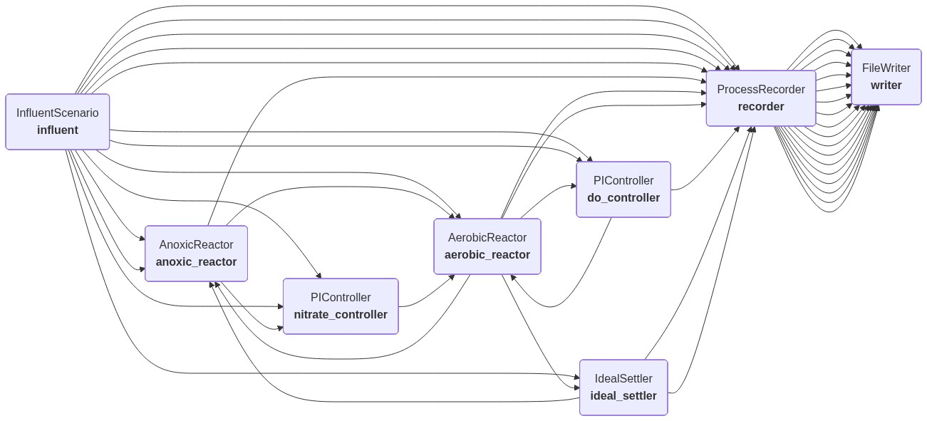
Diagram of the process
The process graph below is generated from the actual LocalProcess wiring. That makes it a useful visual check that the internal recycle, return sludge, controllers, and direct writer connections are connected in the way the code intends.
diagram_url = MermaidDiagram.from_process(process).url
print(diagram_url)
print(markdown_diagram(process))
Inspect the parameter set
The values below are the main operating and controller parameters exposed by the demo model. The dissolved-oxygen controller gains are intentionally softer than the earlier notebook revision, and the aerobic reactor now applies a small slew limit to KLa so the aeration actuator cannot jump unrealistically from one 5-minute sample to the next. That keeps the DO trace easier to read while preserving the basic control story.
parameter_table = pd.DataFrame(
    [
        ("Anoxic volume", params.v_anoxic_m3, "m^3"),
        ("Aerobic volume", params.v_aerobic_m3, "m^3"),
        ("Average influent flow", params.q_in_avg_m3_d, "m^3/d"),
        ("Return sludge flow", params.q_return_m3_d, "m^3/d"),
        ("Internal recycle bias", params.q_internal_bias_m3_d, "m^3/d"),
        ("DO setpoint", params.do_setpoint_g_m3, "g/m^3"),
        ("Nitrate setpoint", params.nitrate_setpoint_g_m3, "g N/m^3"),
        ("KLa bias", params.kla_bias_d_inv, "d^-1"),
        ("KLa slew limit per step", params.kla_rate_limit_d_inv_per_step, "d^-1"),
        ("DO controller Kp", params.do_kp, "-"),
        ("DO controller Ki", params.do_ki, "d^-1"),
        ("Nitrate controller Kp", params.nitrate_kp, "-"),
        ("Nitrate controller Ki", params.nitrate_ki, "d^-1"),
        ("Time step", params.dt_days * 24 * 60, "minutes"),
        ("Simulation horizon", params.total_days, "days"),
    ],
    columns=["Parameter", "Value", "Unit"],
)
parameter_table
Run the simulation
For the run cell we create a fresh process instance so the execution state is clean even if you re-run the notebook sections out of order.
results_path = Path("bsm1_results.csv")
results_path.unlink(missing_ok=True)
process = build_process(output_path=results_path, params=params)
async with process:
    await process.run()
df = pd.read_csv(results_path)
df.head()
Summarize the closed-loop response
Official BSM1 studies often report standardized quality and cost indices. This demo keeps the summary lighter: it looks at average effluent quality and average actuator usage over the final three days of the run.
These numbers are tutorial-scale surrogates rather than benchmark-comparable BSM1 KPIs. They are most useful for checking whether the simplified control story behaves plausibly under the imposed disturbances.
final_window = df[df["time_day_out"] >= (params.total_days - 3.0)]
summary = pd.DataFrame(
    {
        "Metric": [
            "Average effluent COD surrogate (S_S + X_S)",
            "Average effluent soluble substrate",
            "Average effluent ammonium",
            "Average effluent nitrate",
            "Average effluent total nitrogen",
            "Average internal recycle flow",
            "Average KLa",
        ],
        "Value": [
            final_window["effluent_cod"].mean(),
            final_window["effluent_s_s"].mean(),
            final_window["effluent_s_nh"].mean(),
            final_window["effluent_s_no"].mean(),
            final_window["effluent_total_n"].mean(),
            final_window["internal_recycle_flow"].mean(),
            final_window["kla_out"].mean(),
        ],
    }
)
summary
Visualize plant behaviour
The first panel shows the imposed influent disturbances. The middle panels show the controlled states and the controller moves. The last panel tracks the effluent quality variables that are most useful for reading this reduced model.
fig = make_subplots(
    rows=4,
    cols=1,
    shared_xaxes=True,
    vertical_spacing=0.05,
    subplot_titles=(
        "Influent disturbances",
        "Controlled reactor states",
        "Manipulated variables",
        "Effluent quality",
    ),
)

fig.add_trace(
    go.Scatter(x=df["time_day_out"], y=df["influent_flow"], name="Influent flow"),
    row=1,
    col=1,
)
fig.add_trace(
    go.Scatter(x=df["time_day_out"], y=df["influent_s_nh"], name="Influent ammonium"),
    row=1,
    col=1,
)

fig.add_trace(
    go.Scatter(x=df["time_day_out"], y=df["aerobic_s_o"], name="Aerobic DO"),
    row=2,
    col=1,
)
fig.add_trace(
    go.Scatter(
        x=df["time_day_out"],
        y=df["do_setpoint_out"],
        name="DO setpoint",
        line={"dash": "dash"},
    ),
    row=2,
    col=1,
)
fig.add_trace(
    go.Scatter(x=df["time_day_out"], y=df["anoxic_s_no"], name="Anoxic nitrate"),
    row=2,
    col=1,
)
fig.add_trace(
    go.Scatter(
        x=df["time_day_out"],
        y=df["nitrate_setpoint_out"],
        name="Nitrate setpoint",
        line={"dash": "dot"},
    ),
    row=2,
    col=1,
)

fig.add_trace(
    go.Scatter(x=df["time_day_out"], y=df["requested_kla_out"], name="Requested KLa"),
    row=3,
    col=1,
)
fig.add_trace(
    go.Scatter(
        x=df["time_day_out"],
        y=df["kla_out"],
        name="Applied KLa",
        line={"width": 3},
    ),
    row=3,
    col=1,
)
fig.add_trace(
    go.Scatter(
        x=df["time_day_out"],
        y=df["internal_recycle_flow"],
        name="Internal recycle flow",
    ),
    row=3,
    col=1,
)

fig.add_trace(
    go.Scatter(
        x=df["time_day_out"],
        y=df["effluent_cod"],
        name="Effluent COD surrogate",
    ),
    row=4,
    col=1,
)
fig.add_trace(
    go.Scatter(
        x=df["time_day_out"],
        y=df["effluent_s_nh"],
        name="Effluent ammonium",
    ),
    row=4,
    col=1,
)
fig.add_trace(
    go.Scatter(
        x=df["time_day_out"],
        y=df["effluent_total_n"],
        name="Effluent total N",
    ),
    row=4,
    col=1,
)

fig.update_layout(height=1100, width=950, template="plotly_white", legend={"orientation": "h"})
fig.update_xaxes(title_text="Time [days]", row=4, col=1)
fig.update_yaxes(title_text="Influent", row=1, col=1)
fig.update_yaxes(title_text="Controlled states", row=2, col=1)
fig.update_yaxes(title_text="Controller outputs", row=3, col=1)
fig.update_yaxes(title_text="Effluent quality", row=4, col=1)
fig.show()
Interpretation
A few things are worth checking when you run the notebook:
- the internal recycle should move as anoxic nitrate drifts away from its setpoint
- the requested
KLacan still move quickly, but the appliedKLashould ramp more smoothly because the aerobic reactor now enforces a per-step slew limit - the aerobic DO trace should still react to disturbances, but with less sample-to-sample chatter than the earlier direct-actuator version
- effluent ammonium and the COD surrogate should worsen during the imposed load increases, then recover as the controllers respond
- the ideal settler keeps solids handling simple, so this notebook emphasizes biological control and process wiring rather than clarifier hydraulics
This version combines the earlier DO gain reduction with a simple actuator model. The controller still decides how much aeration it wants, but the plant applies that request through a limited-rate KLa change, which is closer to how a real blower or valve train behaves than an instantaneous jump. That makes the plotted trajectories easier to read without changing the tutorial scope of the model.
Treat these trends as qualitative checks on the reduced control topology, not as benchmark-faithful BSM1 performance claims. Natural extensions are adding a more detailed clarifier, splitting the bioreactor back into multiple compartments, or computing official BSM1-style quality and operating-cost indices.