Crusher circuit simulation with Population Balance Modelling
![]()
![]()
This example demonstrates how to build a dynamic crusher circuit simulation using Plugboard, based on the Population Balance Model (PBM) approach widely used in mineral processing.
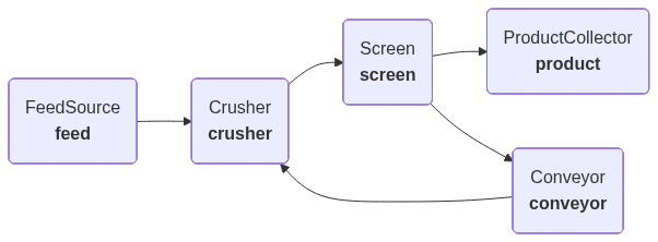
We model a closed-circuit crushing plant with five interconnected components:
- Feed Source — provides raw ore with an initial particle size distribution (PSD)
- Crusher — breaks particles using the Whiten/King crusher model
- Screen — classifies material into undersize (product) and oversize (recirculated)
- Conveyor — introduces a transport delay on the recirculation loop (simulates a conveyor belt)
- Product Collector — accumulates the final product and reports quality metrics
The model tracks how the particle size distribution and mass flow evolve dynamically as the circulating load builds up over time.
Population Balance Model background
The PBM is the standard mathematical framework for modelling comminution (size reduction) processes. For crushers, the Whiten model treats the crushing chamber as a series of classification and breakage stages:
$$P = [B \cdot S + (I - S)] \cdot F$$
where:
- $F$ is the feed size distribution vector
- $P$ is the product size distribution vector
- $S$ is the selection (classification) matrix — probability of a particle being selected for breakage based on crusher geometry
- $B$ is the breakage matrix — distribution of daughter fragments produced when a particle breaks
- $I$ is the identity matrix
Key references:
- Whiten, W.J. (1974). A matrix theory of comminution machines. Chemical Engineering Science, 29(2), 589-599.
- King, R.P. (2001). Modeling and Simulation of Mineral Processing Systems. Butterworth-Heinemann.
- Austin, L.G., Klimpel, R.R., and Luckie, P.T. (1984). Process Engineering of Size Reduction: Ball Milling. SME.
# Install plugboard and dependencies for Google Colab
!pip install -q plugboard plotly
import typing as _t

from pydantic import BaseModel, field_validator

from plugboard.component import Component, IOController as IO
from plugboard.connector import AsyncioConnector
from plugboard.process import LocalProcess
from plugboard.schemas import ComponentArgsDict, ConnectorSpec
Particle Size Distribution data model
We define a custom Pydantic model to represent particle size distributions (PSDs) throughout the circuit. This ensures data validation and provides a clean interface for working with size fractions.
The mass_tonnes field tracks the absolute mass flow of each stream, which is critical for correctly modelling the mass-weighted mixing of fresh feed and recirculated material in the crusher.
class PSD(BaseModel):
    """Particle Size Distribution.

    Tracks the mass fraction retained in each discrete size class,
    together with the absolute mass flow (tonnes) of the stream.

    Size classes are defined by their upper boundary (in mm),
    ordered from coarsest to finest.
    """

    size_classes: list[float]
    mass_fractions: list[float]
    mass_tonnes: float = 1.0

    @field_validator("mass_fractions")
    @classmethod
    def validate_fractions(cls, v: list[float]) -> list[float]:
        total = sum(v)
        if abs(total - 1.0) > 1e-6 and total > 0:
            # Normalise to ensure mass balance
            return [f / total for f in v]
        return v

    def _percentile_size(self, target: float) -> float:
        """Interpolated percentile passing size (mm)."""
        cumulative = 0.0
        for i in range(len(self.size_classes) - 1, -1, -1):
            prev_cum = cumulative
            cumulative += self.mass_fractions[i]
            if cumulative >= target:
                if self.mass_fractions[i] > 0:
                    frac = (target - prev_cum) / self.mass_fractions[i]
                else:
                    frac = 0.0
                lower = self.size_classes[i + 1] if i < len(self.size_classes) - 1 else 0.0
                return lower + frac * (self.size_classes[i] - lower)
        return self.size_classes[0]

    @property
    def d80(self) -> float:
        """80th percentile passing size (mm), interpolated."""
        return self._percentile_size(0.80)

    @property
    def d50(self) -> float:
        """50th percentile passing size (mm), interpolated."""
        return self._percentile_size(0.50)

    def to_cumulative_passing(self) -> list[float]:
        """Return cumulative % passing for each size class."""
        result: list[float] = []
        cumulative = 0.0
        for i in range(len(self.size_classes) - 1, -1, -1):
            cumulative += self.mass_fractions[i]
            result.insert(0, cumulative * 100)
        return result
Crusher model functions
These helper functions implement the Whiten crusher model. The selection function determines which particles are large enough to be broken based on the crusher's closed-side setting (CSS) and open-side setting (OSS). The breakage function describes how broken particles distribute across finer size classes.
def build_selection_vector(
    size_classes: list[float],
    css: float,
    oss: float,
    k3: float = 2.3,
) -> list[float]:
    """Build the crusher selection (classification) vector.

    Implements the Whiten classification function:
    - Particles smaller than CSS pass through unbroken (S=0)
    - Particles larger than OSS are always broken (S=1)
    - Particles between CSS and OSS have a fractional probability

    Args:
        size_classes: Upper bounds of each size class (mm), coarsest first.
        css: Closed-side setting (mm).
        oss: Open-side setting (mm).
        k3: Shape parameter controlling the classification curve steepness.

    Returns:
        Selection probability for each size class.
    """
    selection: list[float] = []
    for d in size_classes:
        if d <= css:
            selection.append(0.0)
        elif d >= oss:
            selection.append(1.0)
        else:
            # Smooth transition between CSS and OSS
            x = (d - css) / (oss - css)
            selection.append(1.0 - (1.0 - x) ** k3)
    return selection


def build_breakage_matrix(
    size_classes: list[float],
    phi: float = 0.4,
    gamma: float = 1.5,
    beta: float = 3.5,
) -> list[list[float]]:
    """Build the breakage distribution matrix (Austin & Luckie, 1972).

    B[i][j] is the fraction of material broken from size class j
    that reports to size class i.

    The cumulative breakage function is:
        B_cum(i,j) = phi * (x_i/x_j)^gamma + (1 - phi) * (x_i/x_j)^beta

    Args:
        size_classes: Upper bounds of each size class (mm), coarsest first.
        phi: Fraction of breakage due to impact (vs. abrasion).
        gamma: Exponent for impact breakage.
        beta: Exponent for abrasion breakage.

    Returns:
        Lower-triangular breakage matrix B[i][j].
    """
    n = len(size_classes)
    B_cum = [[0.0] * n for _ in range(n)]

    for j in range(n):
        for i in range(j, n):
            if i == j:
                B_cum[i][j] = 1.0
            else:
                ratio = size_classes[i] / size_classes[j]
                B_cum[i][j] = phi * ratio**gamma + (1.0 - phi) * ratio**beta

    # Convert cumulative to fractional (incremental) breakage
    B: list[list[float]] = [[0.0] * n for _ in range(n)]
    for j in range(n):
        for i in range(j + 1, n):
            if i == n - 1:
                B[i][j] = B_cum[i][j]
            else:
                B[i][j] = B_cum[i][j] - B_cum[i + 1][j]

    return B


def apply_crusher(feed: PSD, selection: list[float], B: list[list[float]]) -> PSD:
    """Apply one pass of the Whiten crusher model.

    P = [B·S + (I - S)] · F

    Args:
        feed: Input particle size distribution.
        selection: Selection vector (diagonal of S matrix).
        B: Breakage matrix.

    Returns:
        Product particle size distribution (mass_tonnes preserved).
    """
    n = len(feed.size_classes)
    f = feed.mass_fractions
    product = [0.0] * n

    for i in range(n):
        # Material that passes through unbroken
        product[i] += (1.0 - selection[i]) * f[i]
        # Material generated by breakage of coarser classes
        for j in range(i):
            product[i] += B[i][j] * selection[j] * f[j]

    # Normalise to maintain mass balance
    total = sum(product)
    if total > 0:
        product = [p / total for p in product]

    return PSD(
        size_classes=feed.size_classes,
        mass_fractions=product,
        mass_tonnes=feed.mass_tonnes,
    )
Screen model function
The screen partition curve models the probability of a particle passing through the screen. Rather than a perfect cut, it uses a logistic model that accounts for the gradual transition around the cut-point size ($d_{50c}$) and a bypass fraction of fine material that misreports to the oversize stream.
$$E_{\text{undersize}}(d) = \frac{1 - \text{bypass}}{1 + (d / d_{50c})^{\alpha}}$$
This gives exactly 50% passing probability at the cut-point $d_{50c}$, with the sharpness parameter $\alpha$ controlling how steep the transition is (King, 2001).
def screen_partition(
    size_classes: list[float],
    d50c: float,
    alpha: float = 4.0,
    bypass: float = 0.05,
) -> list[float]:
    """Calculate screen partition (efficiency) curve.

    Uses a logistic partition model for the screen. Returns the
    fraction of material in each size class that reports to the
    undersize (product) stream.

    Args:
        size_classes: Upper bounds of each size class (mm), coarsest first.
        d50c: Corrected cut-point size (mm) — 50% partition size.
        alpha: Sharpness of separation (higher = sharper cut).
        bypass: Fraction of fines that misreport to oversize.

    Returns:
        Efficiency (fraction passing to undersize) for each size class.

    References:
        King, R.P. (2001). Modeling and Simulation of Mineral Processing
        Systems, Ch. 8. Butterworth-Heinemann.
    """
    efficiency: list[float] = []
    for d in size_classes:
        e_undersize = (1.0 - bypass) / (1.0 + (d / d50c) ** alpha)
        efficiency.append(e_undersize)
    return efficiency
Plugboard components
Now we define the Plugboard components that make up our crusher circuit:
FeedSource— generates a steady feed of ore with a given PSD and mass flow rate (tonnes per time step)Crusher— applies the Whiten PBM model to produce a finer PSD, using mass-weighted mixing of feed and recirculated materialScreen— splits the crusher product into undersize (product) and oversize (recirculated), tracking mass flow through each streamConveyor— introduces a transport delay on the recirculation loop (simulates a conveyor belt carrying oversize material back to the crusher)ProductCollector— accumulates the final product and reports quality metrics
class FeedSource(Component):
    """Generates a feed stream with a fixed particle size distribution.

    Runs for a set number of time steps, representing batches of ore
    arriving at the crushing circuit.
    """

    io = IO(outputs=["feed_psd"])

    def __init__(
        self,
        size_classes: list[float],
        feed_fractions: list[float],
        feed_tonnes: float = 100.0,
        total_steps: int = 50,
        **kwargs: _t.Unpack[ComponentArgsDict],
    ) -> None:
        super().__init__(**kwargs)
        self._psd = PSD(
            size_classes=size_classes,
            mass_fractions=feed_fractions,
            mass_tonnes=feed_tonnes,
        )
        self._total_steps = total_steps
        self._step_count = 0

    async def step(self) -> None:
        if self._step_count < self._total_steps:
            self.feed_psd = self._psd.model_dump()
            self._step_count += 1
        else:
            await self.io.close()


class Crusher(Component):
    """Whiten/King crusher model.

    Receives a feed PSD (fresh feed combined with recirculated oversize)
    and applies the PBM to produce a crushed product PSD.  Mass-weighted
    mixing ensures the feed-to-recirculation ratio evolves dynamically.

    Parameters:
        css: Closed-side setting (mm) — smallest gap in the crusher.
        oss: Open-side setting (mm) — largest gap in the crusher.
        k3: Classification curve shape parameter.
        phi: Impact fraction in the breakage function.
        gamma: Impact breakage exponent.
        beta: Abrasion breakage exponent.
        n_stages: Number of internal breakage stages (Whiten multi-stage model).
    """

    io = IO(inputs=["feed_psd", "recirc_psd"], outputs=["product_psd"])

    def __init__(
        self,
        css: float = 12.0,
        oss: float = 25.0,
        k3: float = 2.3,
        phi: float = 0.4,
        gamma: float = 1.5,
        beta: float = 3.5,
        n_stages: int = 3,
        **kwargs: _t.Unpack[ComponentArgsDict],
    ) -> None:
        super().__init__(**kwargs)
        self._css = css
        self._oss = oss
        self._k3 = k3
        self._phi = phi
        self._gamma = gamma
        self._beta = beta
        self._n_stages = n_stages
        self._selection: list[float] | None = None
        self._breakage: list[list[float]] | None = None

    async def step(self) -> None:
        feed = PSD(**self.feed_psd)

        # Build matrices on first call (size classes are now known)
        if self._selection is None:
            self._selection = build_selection_vector(
                feed.size_classes, self._css, self._oss, self._k3
            )
            self._breakage = build_breakage_matrix(
                feed.size_classes, self._phi, self._gamma, self._beta
            )

        # Mass-weighted mixing of fresh feed and recirculated oversize
        recirc = self.recirc_psd
        if recirc is not None:
            recirc_psd = PSD(**recirc)
            feed_mass = feed.mass_tonnes
            recirc_mass = recirc_psd.mass_tonnes
            total_mass = feed_mass + recirc_mass
            w_f = feed_mass / total_mass
            w_r = recirc_mass / total_mass
            combined = [
                w_f * f + w_r * r for f, r in zip(feed.mass_fractions, recirc_psd.mass_fractions)
            ]
            feed = PSD(
                size_classes=feed.size_classes,
                mass_fractions=combined,
                mass_tonnes=total_mass,
            )

        # Apply multi-stage crushing
        result = feed
        if self._breakage is None:
            raise RuntimeError("Breakage matrix not initialised")
        for _ in range(self._n_stages):
            result = apply_crusher(result, self._selection, self._breakage)

        self.product_psd = result.model_dump()


class Screen(Component):
    """Vibrating screen separator.

    Splits the crusher product into undersize (product) and oversize
    (recirculated back to the crusher). Tracks mass flow through each
    output stream.

    Parameters:
        d50c: Cut-point size (mm) — particles near this size have 50% chance of passing.
        alpha: Sharpness of the separation curve.
        bypass: Fraction of fines misreporting to oversize.
    """

    io = IO(inputs=["crusher_product"], outputs=["undersize", "oversize"])

    def __init__(
        self,
        d50c: float = 15.0,
        alpha: float = 4.0,
        bypass: float = 0.05,
        **kwargs: _t.Unpack[ComponentArgsDict],
    ) -> None:
        super().__init__(**kwargs)
        self._d50c = d50c
        self._alpha = alpha
        self._bypass = bypass

    async def step(self) -> None:
        feed = PSD(**self.crusher_product)
        efficiency = screen_partition(feed.size_classes, self._d50c, self._alpha, self._bypass)

        undersize_fracs: list[float] = []
        oversize_fracs: list[float] = []
        for i, f in enumerate(feed.mass_fractions):
            undersize_fracs.append(f * efficiency[i])
            oversize_fracs.append(f * (1.0 - efficiency[i]))

        # Mass split: proportion reporting to each stream
        u_total = sum(undersize_fracs)
        o_total = sum(oversize_fracs)

        undersize_mass = feed.mass_tonnes * u_total
        oversize_mass = feed.mass_tonnes * o_total

        if u_total > 0:
            undersize_fracs = [u / u_total for u in undersize_fracs]
        if o_total > 0:
            oversize_fracs = [o / o_total for o in oversize_fracs]

        self.undersize = PSD(
            size_classes=feed.size_classes,
            mass_fractions=undersize_fracs,
            mass_tonnes=undersize_mass,
        ).model_dump()
        self.oversize = PSD(
            size_classes=feed.size_classes,
            mass_fractions=oversize_fracs,
            mass_tonnes=oversize_mass,
        ).model_dump()


class Conveyor(Component):
    """Transport delay for the recirculation loop.

    Simulates a conveyor belt by buffering PSDs in a FIFO queue.
    The output is delayed by `delay_steps` time steps, creating
    realistic transient dynamics in the circuit.

    Parameters:
        delay_steps: Number of time steps to delay the material.
    """

    io = IO(inputs=["input_psd"], outputs=["output_psd"])

    def __init__(
        self,
        delay_steps: int = 3,
        **kwargs: _t.Unpack[ComponentArgsDict],
    ) -> None:
        super().__init__(**kwargs)
        self._delay_steps = delay_steps
        self._buffer: list[dict[str, _t.Any] | None] = [None] * delay_steps

    async def step(self) -> None:
        # Push new material onto the buffer, pop the oldest
        self._buffer.append(self.input_psd)
        delayed = self._buffer.pop(0)
        self.output_psd = delayed


class ProductCollector(Component):
    """Collects the final product stream and tracks quality metrics.

    Records the PSD at each time step and computes running statistics
    including the product d80 (80th percentile passing size).
    """

    io = IO(inputs=["product_psd"], outputs=["d80", "d50"])

    def __init__(
        self,
        target_d80: float = 20.0,
        **kwargs: _t.Unpack[ComponentArgsDict],
    ) -> None:
        super().__init__(**kwargs)
        self._target_d80 = target_d80
        self.psd_history: list[dict[str, _t.Any]] = []

    async def step(self) -> None:
        psd = PSD(**self.product_psd)
        self.psd_history.append(psd.model_dump())
        self.d80 = psd.d80
        self.d50 = psd.d50
Define the size classes and initial feed
We use a standard $\sqrt{2}$ sieve series from 150 mm down to ~4.75 mm, giving 11 size classes. The fresh feed is a typical ROM (run-of-mine) ore distribution with most material in the coarser fractions.
# Standard sqrt(2) sieve series from 150 mm down to ~4.75 mm
SIZE_CLASSES = [150.0, 106.0, 75.0, 53.0, 37.5, 26.5, 19.0, 13.2, 9.5, 6.7, 4.75]

# ROM ore feed distribution (mass fractions, coarsest to finest)
FEED_FRACTIONS = [0.05, 0.10, 0.15, 0.20, 0.18, 0.12, 0.08, 0.05, 0.04, 0.02, 0.01]
Assemble and run the process
The circuit has a recirculation loop: screen oversize passes through a Conveyor (with a 3-step transport delay) before feeding back into the crusher. This delay simulates the time for material to travel on a conveyor belt, and creates realistic transient dynamics as the circulating load builds up.
To break the circular dependency in the loop, we provide initial_values for the recirc_psd input on the Crusher component (set to None on the first step).
Each stream carries its absolute mass flow (in tonnes), so the crusher correctly weights the mixing ratio of fresh feed vs. recirculated oversize.
connect = lambda src, tgt: AsyncioConnector(spec=ConnectorSpec(source=src, target=tgt))

process = LocalProcess(
    components=[
        FeedSource(
            name="feed",
            size_classes=SIZE_CLASSES,
            feed_fractions=FEED_FRACTIONS,
            feed_tonnes=100.0,
            total_steps=50,
        ),
        Crusher(
            name="crusher",
            css=12.0,
            oss=30.0,
            k3=2.3,
            n_stages=2,
            initial_values={"recirc_psd": [None]},
        ),
        Screen(
            name="screen",
            d50c=18.0,
            alpha=3.5,
            bypass=0.05,
        ),
        Conveyor(
            name="conveyor",
            delay_steps=3,
        ),
        ProductCollector(
            name="product",
            target_d80=20.0,
        ),
    ],
    connectors=[
        # Fresh feed → Crusher
        connect("feed.feed_psd", "crusher.feed_psd"),
        # Crusher → Screen
        connect("crusher.product_psd", "screen.crusher_product"),
        # Screen undersize → Product
        connect("screen.undersize", "product.product_psd"),
        # Screen oversize → Conveyor → Crusher (recirculation with delay)
        connect("screen.oversize", "conveyor.input_psd"),
        connect("conveyor.output_psd", "crusher.recirc_psd"),
    ],
)

print(
    f"Crusher circuit created: {len(process.components)} components, {len(process.connectors)} connectors"
)
# Visualise the process as a diagram
from plugboard.diagram import MermaidDiagram

diagram_url = MermaidDiagram.from_process(process).url
print(diagram_url)
# Run the simulation
async with process:
    await process.run()

print("Simulation complete!")
print(f"Final product d80: {process.components['product'].d80:.2f} mm")
print(f"Final product d50: {process.components['product'].d50:.2f} mm")
Visualise results
Let's plot the evolution of the product size metrics and mass flow over time. The conveyor delay creates distinct step-changes in the circulating load, and we can see the circuit gradually approach steady state.
import plotly.graph_objects as go
from plotly.subplots import make_subplots

collector = process.components["product"]
history = collector.psd_history

# Extract metrics
d80_values = [PSD(**h).d80 for h in history]
d50_values = [PSD(**h).d50 for h in history]
mass_values = [PSD(**h).mass_tonnes for h in history]
steps = list(range(1, len(d80_values) + 1))

fig = make_subplots(
    rows=2,
    cols=2,
    subplot_titles=(
        "Product size metrics over time",
        "Product mass flow over time",
        "Final cumulative PSD",
        "Circulating load ratio",
    ),
    vertical_spacing=0.15,
    horizontal_spacing=0.12,
)

# --- Plot 1: d80/d50 evolution ---
fig.add_trace(
    go.Scatter(
        x=steps,
        y=d80_values,
        name="d80",
        line=dict(color="#2196F3", width=2),
    ),
    row=1,
    col=1,
)
fig.add_trace(
    go.Scatter(
        x=steps,
        y=d50_values,
        name="d50",
        line=dict(color="#FF9800", width=2),
    ),
    row=1,
    col=1,
)

# --- Plot 2: Mass flow ---
fig.add_trace(
    go.Scatter(
        x=steps,
        y=mass_values,
        name="Product mass (t)",
        line=dict(color="#4CAF50", width=2),
        fill="tozeroy",
        fillcolor="rgba(76, 175, 80, 0.1)",
    ),
    row=1,
    col=2,
)
fig.add_hline(
    y=100.0,
    line_dash="dash",
    line_color="gray",
    annotation_text="Feed rate (100 t)",
    row=1,
    col=2,
)

# --- Plot 3: Final cumulative PSD ---
final_psd = PSD(**history[-1])
cum_passing = final_psd.to_cumulative_passing()

fig.add_trace(
    go.Scatter(
        x=final_psd.size_classes,
        y=cum_passing,
        name="Cumulative % passing",
        line=dict(color="#9C27B0", width=2),
        marker=dict(size=6),
    ),
    row=2,
    col=1,
)

# --- Plot 4: Circulating load ratio ---
circ_load = [(100.0 - m) / 100.0 * 100 for m in mass_values]
fig.add_trace(
    go.Scatter(
        x=steps,
        y=circ_load,
        name="Circulating load (%)",
        line=dict(color="#F44336", width=2),
    ),
    row=2,
    col=2,
)

fig.update_xaxes(title_text="Time step", row=1, col=1)
fig.update_yaxes(title_text="Size (mm)", row=1, col=1)
fig.update_xaxes(title_text="Time step", row=1, col=2)
fig.update_yaxes(title_text="Mass (tonnes)", row=1, col=2)
fig.update_xaxes(title_text="Particle size (mm)", type="log", row=2, col=1)
fig.update_yaxes(title_text="Cumulative % passing", range=[0, 105], row=2, col=1)
fig.update_xaxes(title_text="Time step", row=2, col=2)
fig.update_yaxes(title_text="Circulating load (%)", row=2, col=2)

fig.update_layout(
    height=700,
    width=1000,
    title_text="Crusher Circuit — Dynamic Simulation Results",
    showlegend=True,
)
fig.show()
import pandas as pd

psd_df = pd.DataFrame(
    {
        "Size (mm)": final_psd.size_classes,
        "Mass %": [frac * 100 for frac in final_psd.mass_fractions],
        "Cum. passing %": cum_passing,
    }
).round({"Size (mm)": 1, "Mass %": 2, "Cum. passing %": 2})

psd_df
Parameter optimisation with the Tuner
Now let's use Plugboard's built-in Tuner to find the optimal crusher and screen settings. The Tuner uses Ray Tune with Optuna to efficiently search the parameter space.
Objective: Minimise the product d80 (we want a finer product).
Parameters to optimise:
- Crusher CSS (6–20 mm): Controls the finest gap of the crusher
- Crusher OSS (20–50 mm): Controls the coarsest gap of the crusher
- Screen cut-point (8–25 mm): Controls where the screen separates undersize from oversize
from plugboard.schemas import (
    FloatParameterSpec,
    ObjectiveSpec,
    ProcessArgsSpec,
    ProcessSpec,
)
from plugboard.tune import Tuner
import crusher_circuit_components  # Import the component classes into the registry for use in the Tuner process spec

# Rebuild the process as a spec using the classes from crusher_circuit.py.
# The Tuner needs to reconstruct the process for each trial, so the component
# types must reference an importable module rather than inline notebook classes.
process_spec = ProcessSpec(
    args=ProcessArgsSpec(
        components=[
            {
                "type": "crusher_circuit_components.FeedSource",
                "args": {
                    "name": "feed",
                    "size_classes": SIZE_CLASSES,
                    "feed_fractions": FEED_FRACTIONS,
                    "feed_tonnes": 100.0,
                    "total_steps": 50,
                },
            },
            {
                "type": "crusher_circuit_components.Crusher",
                "args": {
                    "name": "crusher",
                    "css": 12.0,
                    "oss": 30.0,
                    "k3": 2.3,
                    "n_stages": 2,
                    "initial_values": {"recirc_psd": [None]},
                },
            },
            {
                "type": "crusher_circuit_components.Screen",
                "args": {"name": "screen", "d50c": 18.0, "alpha": 3.5, "bypass": 0.05},
            },
            {
                "type": "crusher_circuit_components.Conveyor",
                "args": {"name": "conveyor", "delay_steps": 3},
            },
            {
                "type": "crusher_circuit_components.ProductCollector",
                "args": {"name": "product", "target_d80": 20.0},
            },
        ],
        connectors=[
            {"source": "feed.feed_psd", "target": "crusher.feed_psd"},
            {"source": "crusher.product_psd", "target": "screen.crusher_product"},
            {"source": "screen.undersize", "target": "product.product_psd"},
            {"source": "screen.oversize", "target": "conveyor.input_psd"},
            {"source": "conveyor.output_psd", "target": "crusher.recirc_psd"},
        ],
    ),
    type="plugboard.process.LocalProcess",
)
tuner = Tuner(
    objective=ObjectiveSpec(
        object_name="product",
        field_type="field",
        field_name="d80",
    ),
    parameters=[
        FloatParameterSpec(
            object_type="component",
            object_name="crusher",
            field_type="arg",
            field_name="css",
            lower=6.0,
            upper=20.0,
        ),
        FloatParameterSpec(
            object_type="component",
            object_name="crusher",
            field_type="arg",
            field_name="oss",
            lower=20.0,
            upper=50.0,
        ),
        FloatParameterSpec(
            object_type="component",
            object_name="screen",
            field_type="arg",
            field_name="d50c",
            lower=8.0,
            upper=25.0,
        ),
    ],
    num_samples=30,
    max_concurrent=4,
    mode="min",
)

result = tuner.run(spec=process_spec)
# Display the optimal parameters found
best_css = result.config["component.crusher.arg.css"]
best_oss = result.config["component.crusher.arg.oss"]
best_d50c = result.config["component.screen.arg.d50c"]
best_d80 = result.metrics["component.product.field.d80"]

print("=" * 50)
print("OPTIMISATION RESULTS")
print("=" * 50)
print(f"  Crusher CSS:      {best_css:.1f} mm")
print(f"  Crusher OSS:      {best_oss:.1f} mm")
print(f"  Screen cut-point: {best_d50c:.1f} mm")
print(f"  Product d80:      {best_d80:.2f} mm")
print("=" * 50)
Summary
This example demonstrated how to:
- Model a physical process — using the Population Balance Model (Whiten/King approach) to simulate crushing and screening
- Use custom data structures — a Pydantic
PSDmodel to track particle size distributions and mass flow with built-in validation - Build a recirculating circuit — using
initial_valuesto break the circular dependency in a closed-loop process - Simulate transport delays — using a
Conveyorcomponent with a FIFO buffer to model conveyor belt transport time - Visualise dynamic behaviour — tracking how the product quality and circulating load evolve over time
- Optimise process parameters — using the
Tunerto search for the crusher and screen settings that produce the finest product
The Whiten crusher model and screen efficiency equations used here are standard tools in mineral processing engineering. For production use, these models would typically be calibrated against plant data from sampling surveys.